14 Tree-Based Models

14.1 Overview of Models on Exam PA

GLM appears on every sitting since 2019.
Decision trees also appear on every version.

Regularized regression (lasso/ridge), bagging, random forests, GBMs appear less frequently (e.g., Dec 2019, Jun 2019).

Priority order:
1. GLM
2. Decision Trees
3. Boosting / Random Forests (when they appear)

Always include this in your executive summary:

After preparing features for modeling, I tested multiple models to identify factors affecting [target]. Each model was trained on 70% of the data (training set) and evaluated on the remaining 30% (test set). This split helps ensure models capture patterns and generalize to new data.

14.2 Bootstrap & Cross-Validation for Hyperparameter Tuning

Bootstrap = resampling with replacement to create many versions of the dataset.

Example: Predicting claim amounts
- Original data has observations A, B, C, D
- Bootstrap sample 1: A, A, B, D → different average claim
- Bootstrap sample 2: C, C, D, D → different average

Repeat hundreds of times → get distribution of parameter estimates (β₀, β₁, …) → compute means, confidence intervals empirically.

Cross-validation (more reliable):

K-fold CV: Divide data into K parts
Train on K-1 folds, test on 1 fold → repeat K times
Average performance across folds

5-fold CV example:
Each fold gives slightly different model (different trees, different β values).
Average smooths out randomness.

14.3 Decision Trees – Core Idea

Goal: Partition feature space into regions with similar target values.

Example: Predict high-cost claim (> $20,000) using age and BMI.

Start with root node
Ask: Age < 20? → Yes/No branches
Then: BMI < 15? → further split
Each terminal (leaf) node gets majority class or average value

Terminology: - Root: top node
- Branches: splits
- Depth/height: number of levels
- Leaf/Terminal nodes: final predictions

Practice exercise (from SRM sample):
Regression tree for log(claim amount) using age_cat and vehicle_age.
Trace three observations through the tree and report predicted values.

14.4 How Trees Choose Splits

Three criteria (only two commonly used on PA):

Gini Index (most common)
- Range: 0 (perfect purity) to 1 (worst)
- Gini = 1 − Σ(pⱼ²) for each class j
- Weighted average across child nodes
Cross-Entropy / Information Gain
- Entropy = −Σ pⱼ log₂(pⱼ)
- Rarely appears on PA, but know definition
Classification Error Rate (almost never used – too insensitive)

Example calculation (two possible splits):
- Split 1: Weighted Gini = 0.49
- Split 2: Weighted Gini = 0.39 → better split

14.5 Complexity Parameter & Pruning

complexity controls tree size (like λ in ridge/lasso).

Loss function:
SSE + complexity × (number of terminal nodes)

Pruning process: - Grow large tree (small complexity)
- Look at complexity table / plot
- Choose complexity that balances error and complexity
- Cut branches with higher complexity

Bias-Variance Tradeoff: - High complexity → simpler tree → high bias, low variance
- Low complexity → complex tree → low bias, high variance

14.6 Advantages & Disadvantages of Single Trees

Advantages: - Easy to interpret
- Built-in variable selection
- Handles categorical variables without dummy encoding
- Captures non-linearities and interactions automatically
- Handles missing values (surrogate splits)

Disadvantages: - Lower predictive accuracy than GLM / lasso / GBM / RF
- Predictions are piecewise constant (step function)
- High variance: small data change → very different tree
- Over-simplifies complex patterns

14.7 Bagging & Random Forests

Bagging = Bootstrap Aggregating
- Fit many trees on different bootstrap samples
- Average predictions (regression) or majority vote (classification)
- Reduces variance, keeps bias similar

Random Forest = Bagged trees + random feature subset at each split
- Extra randomness → more independent trees → lower variance
- Only one main tuning parameter: mtry (features per split)

Advantages: - Resilient to overfitting
- Measures variable importance
- All single-tree benefits

Disadvantages: - Harder to interpret
- Struggles with severe class imbalance (need stratified sampling / oversampling)
- Lower accuracy than boosting
- Cannot extrapolate beyond training range (regression)

14.8 Boosted Trees (GBM)

Boosting: sequential trees, each fits residuals of previous.

Process: 1. Start with mean(target)
2. Fit tree to residuals → get predictions
3. Update: new target = previous residuals − learning_rate × tree prediction
4. Repeat

Key parameters: - Learning rate (shrinkage)
- Number of trees
- Tree depth / interaction.depth
- Subsample fraction

Advantages: - Highest predictive accuracy on many problems
- Handles non-linearities, interactions, missing values, outliers
- Widely used in actuarial modeling and Kaggle winners

Disadvantages: - Requires larger sample size
- Longer training time
- Easy to overfit → needs careful tuning / CV

14.9 Partial Dependence Plots

Show marginal effect of one (or two) predictors after averaging out others.

Useful for explaining: “How does age affect predicted charges, holding everything else constant?”

14.10 Final Exam Tips

Know definitions: pruning, bagging, boosting, Gini, entropy, complexity
Be ready to interpret tree output (splits, leaf values, % in each node)
Compare models: interpretability vs accuracy
Write concisely: “Random Forest averages many bagged trees to reduce variance. Boosting builds trees sequentially on residuals for higher accuracy but risks overfitting.”

For 2026 practice exams + solutions:
https://www.PredictiveInsightsAI.com

14.11 Load Dataset

datasets <- import("datasets")
ds <- datasets$load_dataset("supersam7/health_costs")
df <- as_tibble(ds$train$to_pandas())
glimpse(df)

## Rows: 1,338
## Columns: 7
## $ age      <dbl> 19, 18, 28, 33, 32, 31, 46, 37, 37, 60, 25, 62, 23, 56, 27, 1…
## $ sex      <chr> "female", "male", "male", "male", "male", "female", "female",…
## $ bmi      <dbl> 27.900, 33.770, 33.000, 22.705, 28.880, 25.740, 33.440, 27.74…
## $ children <dbl> 0, 1, 3, 0, 0, 0, 1, 3, 2, 0, 0, 0, 0, 0, 0, 1, 1, 0, 0, 0, 0…
## $ smoker   <chr> "yes", "no", "no", "no", "no", "no", "no", "no", "no", "no", …
## $ region   <chr> "southwest", "southeast", "southeast", "northwest", "northwes…
## $ charges  <dbl> 16884.924, 1725.552, 4449.462, 21984.471, 3866.855, 3756.622,…

14.12 Single Decision Tree

tree_model <- rpart(charges ~ age + bmi + smoker + children + region,
                    data = df, method = "anova",
                    control = rpart.control(minsplit = 20, cp = 0.001))
rpart.plot(tree_model, type = 3, extra = 101,
           main = "Decision Tree – Charges 2026")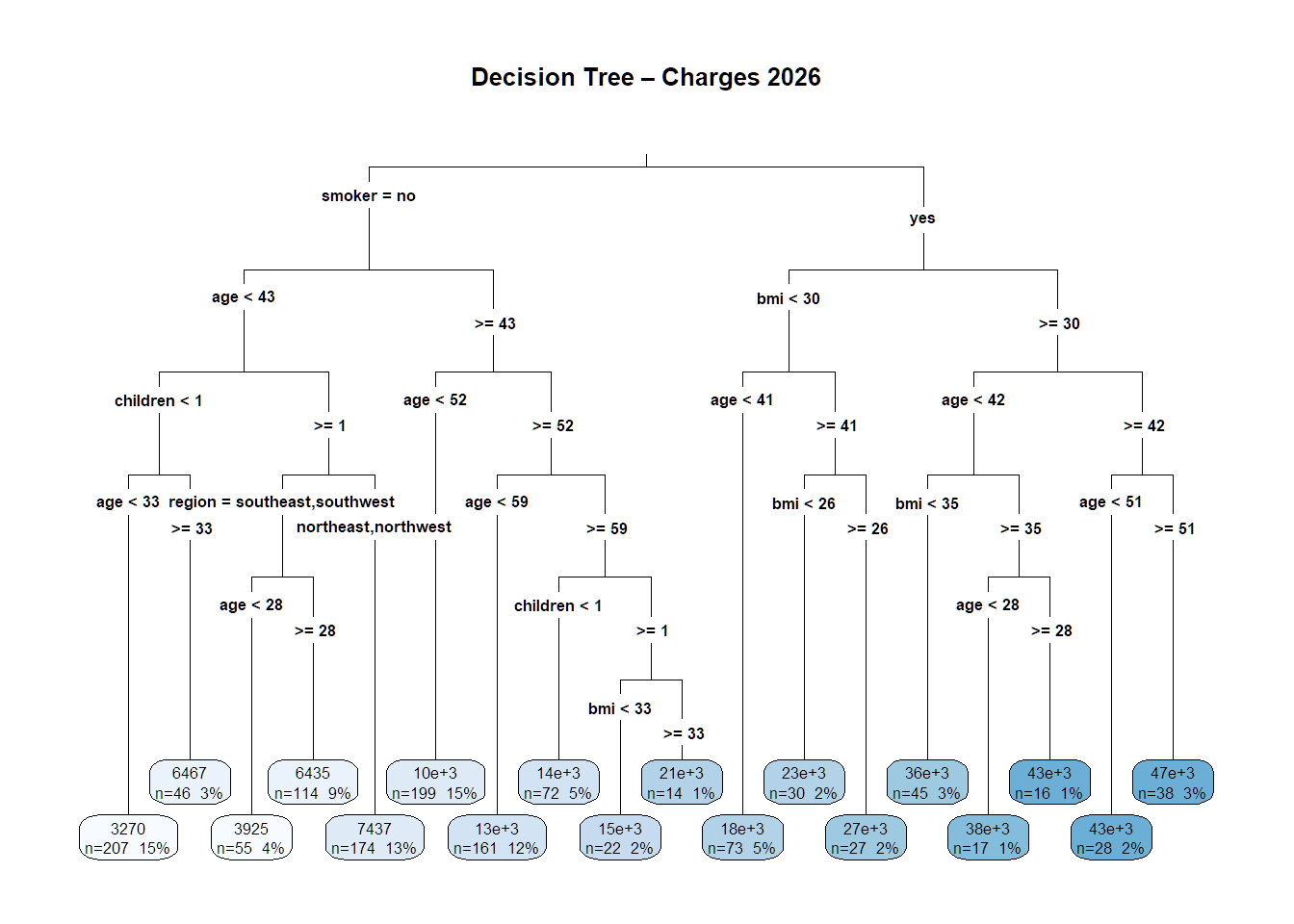

14.13 Random Forest

set.seed(42)
train_idx <- createDataPartition(df$charges, p = 0.8, list = FALSE)
train <- df[train_idx, ]
test <- df[-train_idx, ]
rf_control <- trainControl(method = "cv", number = 5)
rf_model <- train(charges ~ ., data = train,
                  method = "rf", trControl = rf_control,
                  tuneLength = 5, ntree = 100)
print(rf_model)

## Random Forest 
## 
## 1072 samples
##    6 predictor
## 
## No pre-processing
## Resampling: Cross-Validated (5 fold) 
## Summary of sample sizes: 857, 858, 857, 858, 858 
## Resampling results across tuning parameters:
## 
##   mtry  RMSE      Rsquared   MAE     
##   2     5220.551  0.8474560  3588.339
##   3     4557.605  0.8590567  2714.177
##   5     4509.468  0.8596150  2522.385
##   6     4532.766  0.8579675  2513.280
##   8     4602.214  0.8541628  2570.483
## 
## RMSE was used to select the optimal model using the smallest value.
## The final value used for the model was mtry = 5.

14.14 Gradient Boosting (gbm)

gbm_control <- trainControl(method = "cv", number = 5)
gbm_grid <- expand.grid(n.trees = c(100, 300),
                        interaction.depth = c(3, 5),
                        shrinkage = c(0.01, 0.1),
                        n.minobsinnode = c(10))
gbm_model <- train(charges ~ ., data = train,
                   method = "gbm", trControl = gbm_control,
                   tuneGrid = gbm_grid, verbose = FALSE)
print(gbm_model)

## Stochastic Gradient Boosting 
## 
## 1072 samples
##    6 predictor
## 
## No pre-processing
## Resampling: Cross-Validated (5 fold) 
## Summary of sample sizes: 859, 857, 857, 858, 857 
## Resampling results across tuning parameters:
## 
##   shrinkage  interaction.depth  n.trees  RMSE      Rsquared   MAE     
##   0.01       3                  100      6283.666  0.8497361  4702.726
##   0.01       3                  300      4460.758  0.8706725  2712.659
##   0.01       5                  100      6088.864  0.8667520  4600.524
##   0.01       5                  300      4350.976  0.8742149  2553.885
##   0.10       3                  100      4329.199  0.8719095  2399.529
##   0.10       3                  300      4519.625  0.8607597  2629.157
##   0.10       5                  100      4398.602  0.8678141  2450.273
##   0.10       5                  300      4650.457  0.8528952  2769.422
## 
## Tuning parameter 'n.minobsinnode' was held constant at a value of 10
## RMSE was used to select the optimal model using the smallest value.
## The final values used for the model were n.trees = 100, interaction.depth =
##  3, shrinkage = 0.1 and n.minobsinnode = 10.

14.15 XGBoost

X_train <- model.matrix(charges ~ . -1, data = train)
X_test <- model.matrix(charges ~ . -1, data = test)
y_train <- train$charges
y_test <- test$charges
xgb_grid <- expand.grid(nrounds = c(200),
                        max_depth = c(3, 6),
                        eta = c(0.05, 0.1),
                        gamma = 0,
                        colsample_bytree = 0.8,
                        min_child_weight = 1,
                        subsample = 0.8)
xgb_model <- train(x = X_train, y = y_train,
                   method = "xgbTree",
                   trControl = trainControl(method = "cv", number = 5),
                   tuneGrid = xgb_grid,
                   verbosity = 0)
print(xgb_model)

## eXtreme Gradient Boosting 
## 
## 1072 samples
##    9 predictor
## 
## No pre-processing
## Resampling: Cross-Validated (5 fold) 
## Summary of sample sizes: 857, 859, 857, 857, 858 
## Resampling results across tuning parameters:
## 
##   eta   max_depth  RMSE      Rsquared   MAE     
##   0.05  3          4390.945  0.8687443  2382.847
##   0.05  6          4777.860  0.8450791  2746.262
##   0.10  3          4540.453  0.8602340  2514.052
##   0.10  6          5023.069  0.8294898  3024.766
## 
## Tuning parameter 'nrounds' was held constant at a value of 200
## Tuning
## 
## Tuning parameter 'min_child_weight' was held constant at a value of 1
## 
## Tuning parameter 'subsample' was held constant at a value of 0.8
## RMSE was used to select the optimal model using the smallest value.
## The final values used for the model were nrounds = 200, max_depth = 3, eta
##  = 0.05, gamma = 0, colsample_bytree = 0.8, min_child_weight = 1 and
##  subsample = 0.8.

14.16 Direct lightgbm

# Manual CV for LightGBM
dtrain <- lgb.Dataset(X_train, label = y_train)
set.seed(42)
folds <- createFolds(y_train, k=5)

params_list <- expand.grid(
  max_depth = c(3,6,8),
  num_leaves = c(20,31,50),
  learning_rate = c(0.1)
)

rmse_results <- numeric(nrow(params_list))

for(i in 1:nrow(params_list)) {
  params <- list(
    objective = "regression",
    metric = "rmse",
    max_depth = params_list$max_depth[i],
    num_leaves = params_list$num_leaves[i],
    learning_rate = params_list$learning_rate[i],
    feature_fraction = 0.8,
    bagging_fraction = 0.8,
    bagging_freq = 5,
    verbose = -1
  )
  
  cv_rmse <- 0
  for(fold_idx in folds) {
    train_fold <- lgb.Dataset(X_train[-fold_idx,], label = y_train[-fold_idx])
    val_fold <- lgb.Dataset(X_train[fold_idx,], label = y_train[fold_idx])
    
    model <- lgb.train(params, train_fold, nrounds=200, valids=list(val=val_fold), early_stopping_rounds=20, verbose=0)
    pred <- predict(model, X_train[fold_idx,])
    cv_rmse <- cv_rmse + sqrt(mean((pred - y_train[fold_idx])^2))
  }
  
  rmse_results[i] <- cv_rmse / 5
}

# Best
best_i <- which.min(rmse_results)
best_params <- params_list[best_i,]
print(best_params)  # Fix: use print

# Final train
lgb_model <- lgb.train(as.list(best_params), dtrain, nrounds=200, valids=list(test=dtest), early_stopping_rounds=20, verbose=0)
print(lgb_model)

14.17 Variable Importance (from direct LightGBM)

lgb.importance(lgb_direct) %>%
  head(15) %>%
  lgb.plot.importance(main = "LightGBM Feature Importance 2026")

Data exploration