Data Load
reticulate::use_python("C:/Users/casti/AppData/Local/Programs/Python/Python313/python.exe", required = TRUE)
Sys.setenv(RETICULATE_UV_ENABLED = "0")

datasets <- import("datasets")
ds <- datasets$load_dataset("supersam7/foot_traffic")
df <- as_tibble(ds["train"]$to_pandas())
glimpse(df)
## Rows: 11,373
## Columns: 7
## $ pedestrians   <dbl> 3172, 14, 10, 521, 126, 2628, 1602, 23, 37, 2709, 2271, …
## $ weather       <chr> "clear-day", "partly-cloudy-night", "partly-cloudy-night…
## $ temperature   <dbl> 44, 41, 36, 76, 35, 73, 48, 32, 57, 41, 81, 44, 87, 67, …
## $ precipitation <dbl> 0.0000, 0.0000, 0.0000, 0.0087, 0.0000, 0.0000, 0.0000, …
## $ hour          <dbl> 14, 21, 21, 9, 6, 19, 15, 21, 21, 15, 13, 9, 13, 22, 14,…
## $ weekday       <chr> "Wednesday", "Sunday", "Thursday", "Tuesday", "Monday", …
## $ temp_forecast <dbl> 37.11765, 41.17647, 40.17647, 75.76471, 50.05882, 70.764…
Task 1: Explore Variables
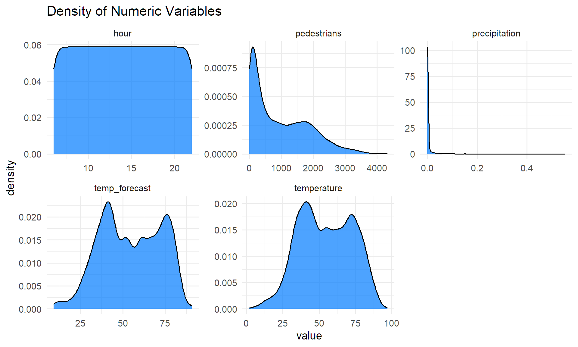
# Numeric variables density
df %>% select_if(is.numeric) %>%
  pivot_longer(everything()) %>%
  ggplot(aes(value)) + geom_density(fill = "#007bff", alpha = 0.7) +
  facet_wrap(~name, scales = "free") + labs(title = "Density of Numeric Variables")
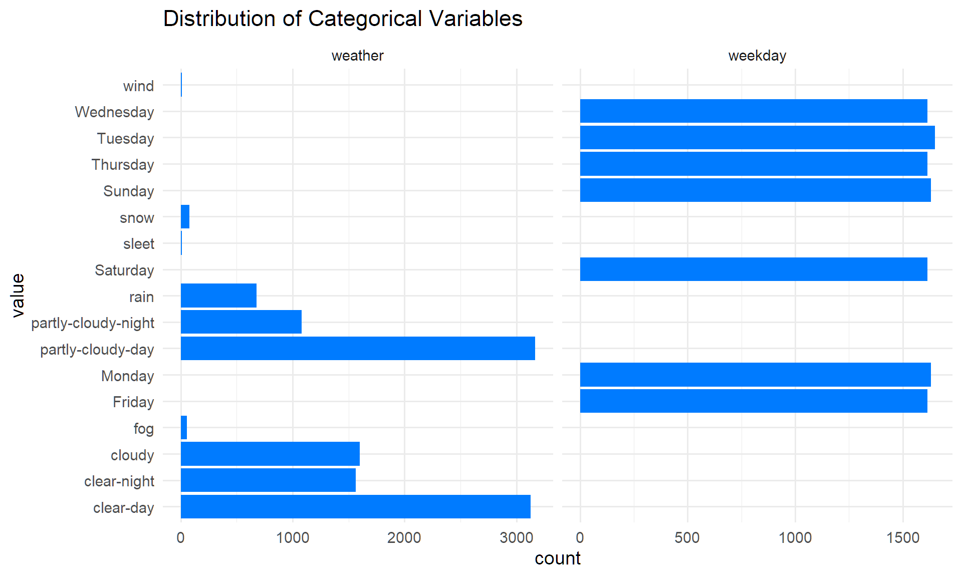
# Categorical variables
df %>% select_if(is.character) %>%
  pivot_longer(everything()) %>%
  ggplot(aes(value)) + geom_bar(fill = "#007bff") +
  facet_wrap(~name, scales = "free_x") + coord_flip() +
  labs(title = "Distribution of Categorical Variables")
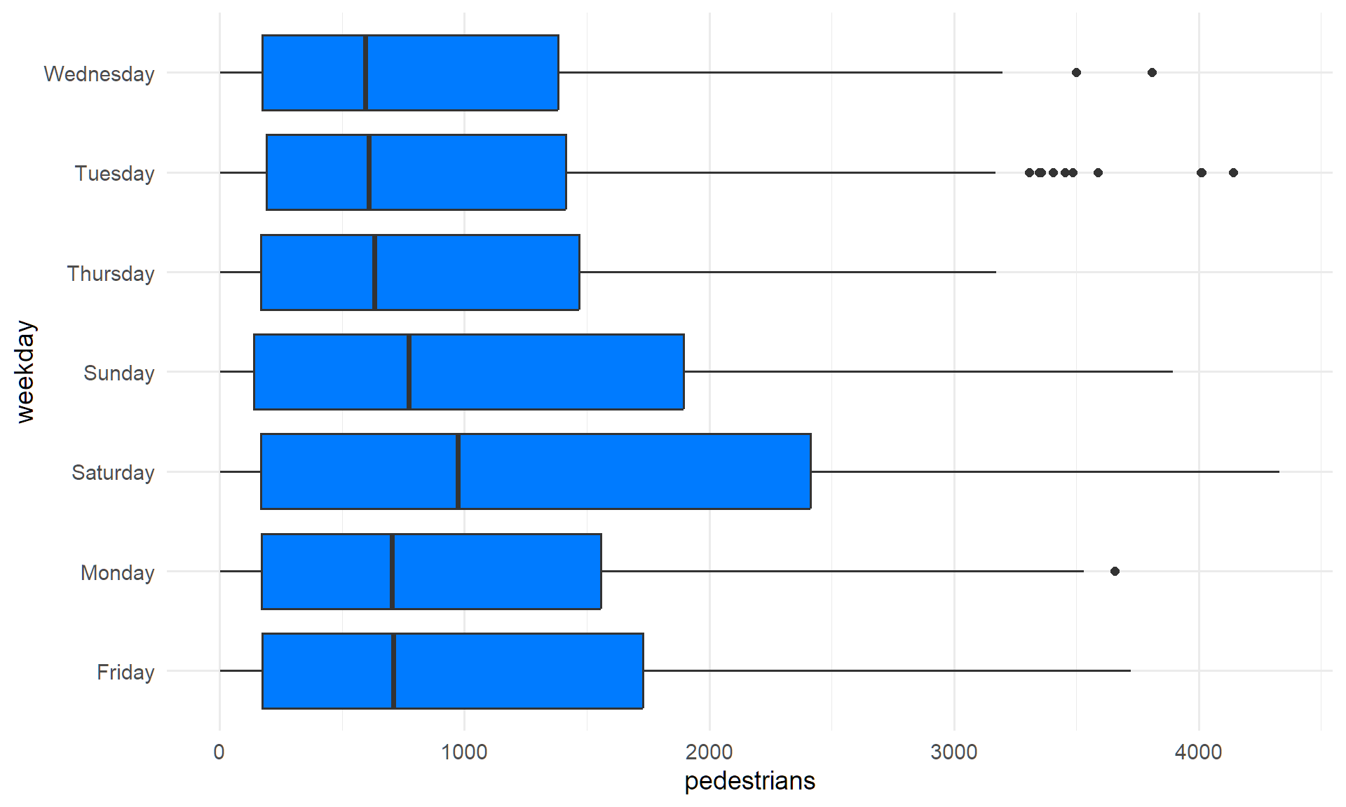
# Pedestrians vs key factors
ggplot(df, aes(weekday, pedestrians)) + geom_boxplot(fill = "#007bff") + coord_flip()
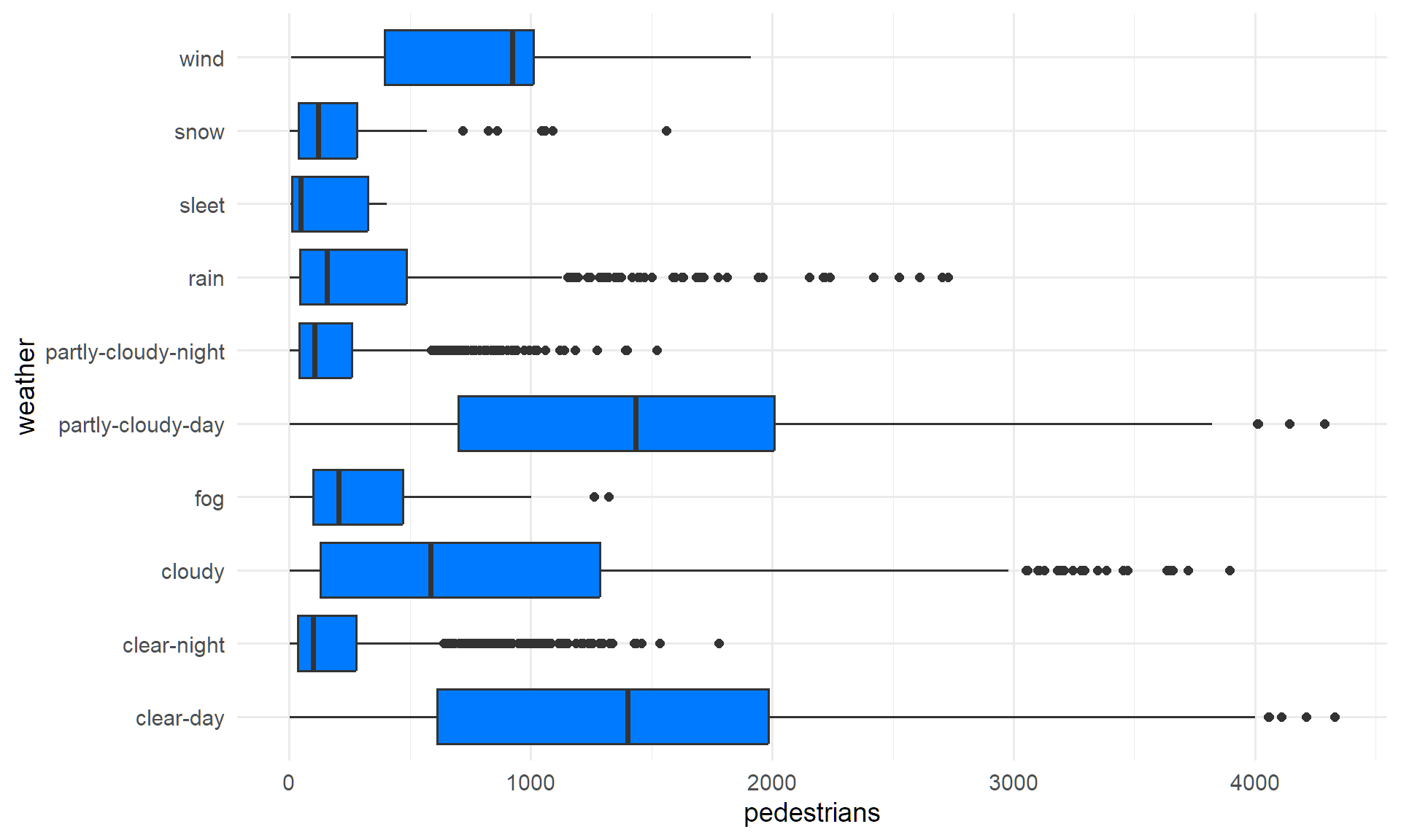
ggplot(df, aes(weather, pedestrians)) + geom_boxplot(fill = "#007bff") + coord_flip()
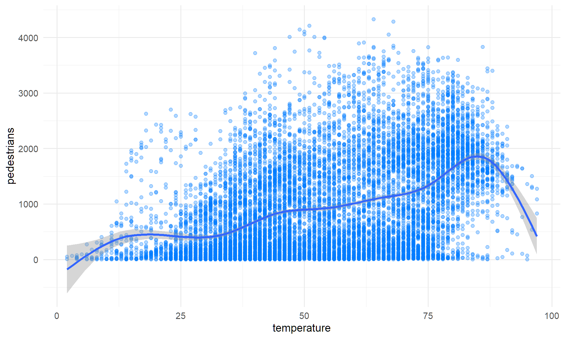
ggplot(df, aes(temperature, pedestrians)) + geom_point(alpha = 0.3, color = "#007bff") + geom_smooth()
Task 2: Reduce Factor Levels
# Weekday: Weekend vs Weekday
df$weekday <- fct_collapse(df$weekday,
  Weekend = c("Saturday", "Sunday"),
  Weekday = c("Monday", "Tuesday", "Wednesday", "Thursday", "Friday"))

# Weather: simplified
df$weather <- fct_collapse(df$weather,
  "Nice" = c("clear-day", "partly-cloudy-day", "clear-night", "partly-cloudy-night"),
  "Rain" = "rain",
  "Bad" = c("fog", "sleet", "snow", "wind", "cloudy"))

table(df$weekday)
##
## Weekday Weekend
##    8126    3247
##
## Nice  Bad Rain
## 8942 1752  679
Task 7: GLM (Poisson & Gamma)
glm_pois <- glm(pedestrians ~ . - ped_sqrt, family = poisson(link = "log"), data = train)
glm_gamma <- glm(pedestrians ~ . - ped_sqrt, family = Gamma(link = "log"), data = train)

rmse_pois <- rmse(test$pedestrians, predict(glm_pois, test, type = "response"))
rmse_gamma <- rmse(test$pedestrians, predict(glm_gamma, test, type = "response"))

cat("Poisson GLM Test RMSE:", rmse_pois, "\n")
## Poisson GLM Test RMSE: 550.9564
cat("Gamma GLM Test RMSE:", rmse_gamma, "\n")
## Gamma GLM Test RMSE: 953.4377
Task 8: Interaction (hour_dist * weather)
glm_int <- glm(pedestrians ~ . - ped_sqrt + hour_dist * weather,
               family = poisson(link = "log"), data = train)
summary(glm_int)
##
## Call:
## glm(formula = pedestrians ~ . - ped_sqrt + hour_dist * weather,
##     family = poisson(link = "log"), data = train)
##
## Coefficients:
##                         Estimate Std. Error  z value Pr(>|z|)
## (Intercept)            6.990e+00  1.325e-03  5276.53   <2e-16 ***
## weatherBad            -1.445e-01  1.616e-03   -89.43   <2e-16 ***
## weatherRain           -6.015e-01  4.120e-03  -145.99   <2e-16 ***
## precipitation         -6.875e+00  4.633e-02  -148.39   <2e-16 ***
## weekdayWeekend         2.954e-01  7.094e-04   416.45   <2e-16 ***
## hour_dist             -2.877e-01  1.685e-04 -1707.14   <2e-16 ***
## temp_use               1.467e-02  1.949e-05   752.64   <2e-16 ***
## weatherBad:hour_dist  -3.375e-02  4.898e-04   -68.90   <2e-16 ***
## weatherRain:hour_dist -2.293e-02  1.056e-03   -21.71   <2e-16 ***
## ---
## Signif. codes:  0 '***' 0.001 '**' 0.01 '*' 0.05 '.' 0.1 ' ' 1
##
## (Dispersion parameter for poisson family taken to be 1)
##
##     Null deviance: 7827274  on 9100  degrees of freedom
## Residual deviance: 2617719  on 9092  degrees of freedom
## AIC: 2689817
##
## Number of Fisher Scoring iterations: 5
rmse_int <- rmse(test$pedestrians, predict(glm_int, test, type = "response"))
cat("GLM with Interaction Test RMSE:", rmse_int, "\n")
## GLM with Interaction Test RMSE: 549.4676
Task 9: Feature Selection (BIC backward)
glm_full <- glm(pedestrians ~ . - ped_sqrt + hour_dist * weather,
                family = poisson(link = "log"), data = train)

glm_bic <- stepAIC(glm_full, direction = "backward", k = log(nrow(train)))
## Start:  AIC=2689881
## pedestrians ~ (weather + precipitation + weekday + hour_dist +
##     temp_use + ped_sqrt) - ped_sqrt + hour_dist * weather
##
##                     Df Deviance     AIC
## <none>                  2617719 2689881
## - weather:hour_dist  2  2622864 2695008
## - precipitation      1  2647396 2719549
## - weekday            1  2785610 2857762
## - temp_use           1  3202377 3274529
##
## Call:
## glm(formula = pedestrians ~ (weather + precipitation + weekday +
##     hour_dist + temp_use + ped_sqrt) - ped_sqrt + hour_dist *
##     weather, family = poisson(link = "log"), data = train)
##
## Coefficients:
##                         Estimate Std. Error  z value Pr(>|z|)
## (Intercept)            6.990e+00  1.325e-03  5276.53   <2e-16 ***
## weatherBad            -1.445e-01  1.616e-03   -89.43   <2e-16 ***
## weatherRain           -6.015e-01  4.120e-03  -145.99   <2e-16 ***
## precipitation         -6.875e+00  4.633e-02  -148.39   <2e-16 ***
## weekdayWeekend         2.954e-01  7.094e-04   416.45   <2e-16 ***
## hour_dist             -2.877e-01  1.685e-04 -1707.14   <2e-16 ***
## temp_use               1.467e-02  1.949e-05   752.64   <2e-16 ***
## weatherBad:hour_dist  -3.375e-02  4.898e-04   -68.90   <2e-16 ***
## weatherRain:hour_dist -2.293e-02  1.056e-03   -21.71   <2e-16 ***
## ---
## Signif. codes:  0 '***' 0.001 '**' 0.01 '*' 0.05 '.' 0.1 ' ' 1
##
## (Dispersion parameter for poisson family taken to be 1)
##
##     Null deviance: 7827274  on 9100  degrees of freedom
## Residual deviance: 2617719  on 9092  degrees of freedom
## AIC: 2689817
##
## Number of Fisher Scoring iterations: 5