9 GLMs for classification
For classification, the predicted values need to be a category instead of a number. Using a discrete target distribution ensures that this will be the case. The probability of an event occurring is \(E[Y] = p\). Unlike the continuous case, all of the link functions have the same range between 0 and 1 because this is a probability.
9.1 Binary target
When \(Y\) is binary, then the Binomial distribution is the only choice. If there are multiple categories, then the Multinomial should be used.
9.2 Count target
When \(Y\) is a count, the Poisson distribution is the only choice. Two examples are counting the number of claims a policy has in a given year or counting the number of people visiting the ER in a given month. The key ingredients are 1) some events and 2) some fixed periods.
Statistically, the name for this is a Poisson Process, which describes a series of discrete events where the average time between events is known, called the “rate” \(\lambda\), but the exact timing of events is unknown. For a time interval of length \(m\), the expected number of events is \(\lambda m\).
By using a GLM, we can fit a different rate for each observation. In the ER example, each patient would have a different rate. Those who are unhealthy or who work in risky environments would have a higher rate of ER visits than those who are healthy and work in offices.
\[Y_i|X_i \sim \text{Poisson}(\lambda_i m_i)\]
When all observations have the same exposure, \(m = 1\). When the mean of the data is far from the variance, an additional parameter known as the dispersion parameter is used. A classic example is when modeling insurance claim counts, which have a lot of zero claims. Then the model is said to be an “over-dispersed Poisson” or “zero-inflated” model.
9.3 Link functions
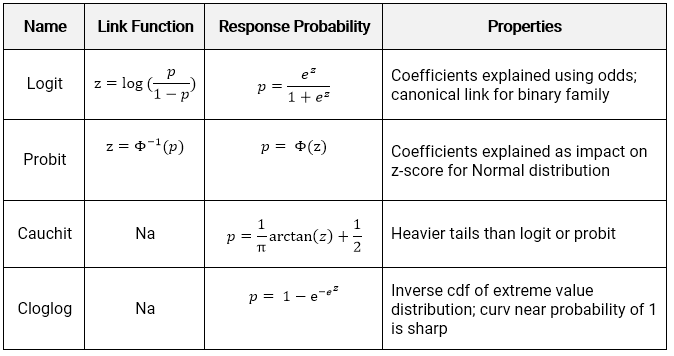
There are four link functions. The most common are the Logit and Probit, but the Cauchit and Cloglog have appeared on the Hospital Readmissions practice exam. The identity link does not make sense for classification because it would result in predictions being outside of \((0,1)\)
9.4 GLM – Poisson / Gamma for Claims
9.5 Penalized Regression – Ridge / Lasso
# Prepare matrix
X <- model.matrix(charges ~ age + bmi + smoker + region + children - 1, data = df)
y <- df$charges

# Lasso (alpha=1)
lasso_fit <- cv.glmnet(X, y, alpha = 1, family = "gaussian")
plot(lasso_fit)
title("Lasso CV – Predictive Insights 2026", col.main = "#00d4ff")

# Best lambda
best_lambda <- lasso_fit$lambda.min
coef(lasso_fit, s = best_lambda)9.6 Interpretation of coefficients
Interpreting the coefficients in classification is trickier than in classification because the result must always be within \((0,1)\).
9.6.1 Logit
The link function \(log(\frac{p}{1-p})\) is known as the log-odds, where the odds are \(\frac{p}{1-p}\). These come up in gambling, where bets are placed on the odds of some event occurring. For example: if the probability of a claim is \(p = 0.8\), then the probability of no claim is 0.2 and the odds of a claim occurring are 0.8/0.2 = 4.
The transformation from probability to odds is monotonic. This is a fancy way of saying that if \(p\) increases, then the odds of \(p\) increases as well, and vice versa if \(p\) decreases. The log transform is monotonic as well.
The net result is that when a variable increases the linear predictor, this increases the log odds, increasing the log of the odds, and vice versa if the linear predictor decreases. In other words, the signs of the coefficients indicate whether the variable increases or decreases the probability of the event.