18 Robocalls Consumer Protections
Simulates a dataset to educate on safe customer phone services, raise awareness against AI/robocall harassment by corporations, and help optimize compliant calling practices. Based on adult dataset stats with added legal/compliance features. Features
Customer demographics (age, education, marital, occupation, etc.) Economic indicators (CPI, CCI, irate, employment) Call details (robot/human calls, 800 number) Location/legal (countries, cities, states, GDPR) Purchase outcome with correlations Usage
Run simulation.py to generate simulated_customer_robocall_dataset.csv. Load in data analysis tools (e.g., R/Python) for modeling. Data Generation
Size: ~48k rows Correlations: Purchase influenced by age, education, cap_gain, robot_calling (negative) Missing values: Simulated in edu_years, housing, job, marital
18.1 GDPR Section
GDPR (General Data Protection Regulation) applies to personal data processing for EU residents or by EU-based entities. For robocalls, it requires explicit consent for automated marketing calls. Non-compliance can lead to fines up to 4% of global turnover. In this dataset, ‘GDPR_applies’ flags cases where GDPR rules must be followed, helping model compliant practices vs. potential harassment in non-regulated areas.
18.2 Deepfake Concerns
Modern robocalls may use deepfake AI voices, mimicking humans so convincingly that recipients can’t tell if it’s automated. This blurs lines between robot/human calls, enabling manipulation/scams. The dataset’s ‘robot_calling’ flag simulates this; in reality, detection tools are needed. Awareness helps consumers report suspicious calls to authorities like FCC/FTC.
# Load needed libraries.
library(ggplot2)
library(dplyr)
library(tidyr)
library(caret)
knitr::opts_chunk$set(warning = FALSE, message = FALSE, fig.width = 10, fig.height = 6)
reticulate::use_python("C:/Users/casti/AppData/Local/Programs/Python/Python313/python.exe", required = TRUE)
# 3. Restart R session inside RStudio
Sys.setenv(RETICULATE_UV_ENABLED = "0")

#.rs.restartR()

library(reticulate)
datasets <- import("datasets")
ds <- datasets$load_dataset("supersam7/robocalls_consumer_protections")
df <- as_tibble(ds["train"]$to_pandas())
summary(df)
## age education_num marital_status occupation
## Min. :17.00 Min. : 1.00 Length:48842 Length:48842
## 1st Qu.:31.00 1st Qu.: 8.00 Class :character Class :character
## Median :39.00 Median :10.00 Mode :character Mode :character
## Mean :39.82 Mean : 9.51
## 3rd Qu.:48.00 3rd Qu.:11.00
## Max. :89.00 Max. :15.00
## cap_gain hours_per_week score value_flag
## Min. : 0 Min. : 1.00 Min. :44.89 Length:48842
## 1st Qu.: 310 1st Qu.:31.00 1st Qu.:57.55 Class :character
## Median : 744 Median :40.00 Median :60.23 Mode :character
## Mean : 1075 Mean :39.93 Mean :60.24
## 3rd Qu.: 1488 3rd Qu.:48.00 3rd Qu.:62.95
## Max. :11599 Max. :98.00 Max. :75.37
## country_of_business country_of_customer state_of_customer city_of_customer
## Length:48842 Length:48842 Length:48842 Length:48842
## Class :character Class :character Class :character Class :character
## Mode :character Mode :character Mode :character Mode :character
##
##
##
## GDPR_applies robot_calling number_of_robot_calls number_of_human_calls
## Min. :0.0000 Min. :0.000 Min. : 0.0000 Min. : 0.000
## 1st Qu.:1.0000 1st Qu.:0.000 1st Qu.: 0.0000 1st Qu.: 2.000
## Median :1.0000 Median :0.000 Median : 0.0000 Median : 3.000
## Mean :0.7518 Mean :0.296 Mean : 0.8822 Mean : 2.993
## 3rd Qu.:1.0000 3rd Qu.:1.000 3rd Qu.: 2.0000 3rd Qu.: 4.000
## Max. :1.0000 Max. :1.000 Max. :10.0000 Max. :12.000
## 800_number_or_not housing loan phone_type
## Min. :0.0000 Length:48842 Length:48842 Length:48842
## 1st Qu.:0.0000 Class :character Class :character Class :character
## Median :1.0000 Mode :character Mode :character Mode :character
## Mean :0.7028
## 3rd Qu.:1.0000
## Max. :1.0000
## month weekday CPI CCI
## Length:48842 Length:48842 Min. :92.20 Min. :-50.80
## Class :character Class :character 1st Qu.:93.18 1st Qu.:-43.65
## Mode :character Mode :character Median :93.57 Median :-40.39
## Mean :93.56 Mean :-40.32
## 3rd Qu.:93.96 3rd Qu.:-37.11
## Max. :94.77 Max. :-26.91
## irate employment purchase
## Min. :0.6481 Min. :4969 Min. :0.0000
## 1st Qu.:2.8917 1st Qu.:5128 1st Qu.:0.0000
## Median :3.5226 Median :5159 Median :0.0000
## Mean :3.4693 Mean :5156 Mean :0.3425
## 3rd Qu.:4.1209 3rd Qu.:5188 3rd Qu.:1.0000
## Max. :5.0450 Max. :5227 Max. :1.0000# Fixed and improved plots for robot calls
# 1. Scatterplot of robot calls vs human calls (with transparency for density)
df |>
ggplot(aes(x = number_of_robot_calls, y = number_of_human_calls)) +
geom_point(alpha = 0.1, color = "#007bff") +
theme_minimal(base_size = 16) +
labs(title = "Robot Calls vs Human Calls", x = "Number of Robot Calls", y = "Number of Human Calls") +
theme(text = element_text(color = "#0056b3"))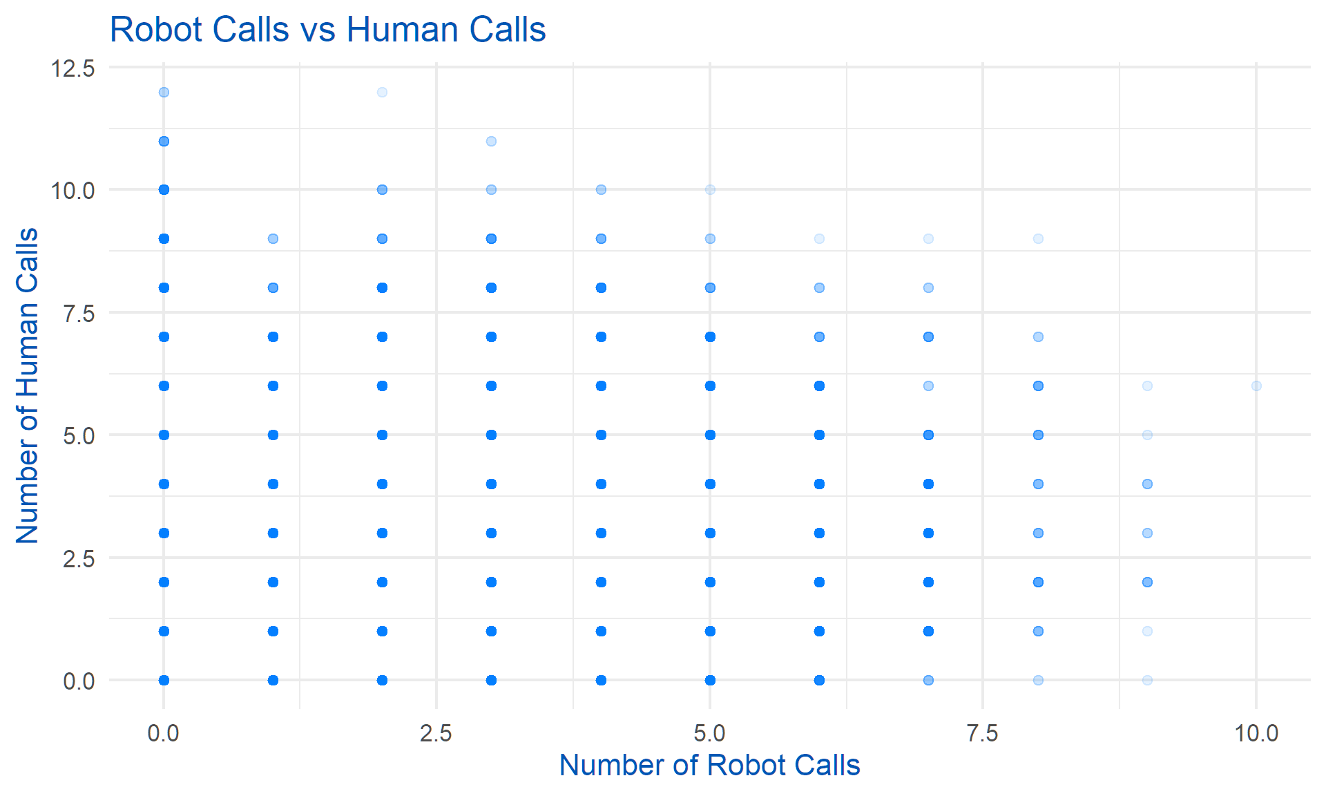
# 2. Histogram of number of robot calls (fixed syntax, added bins)
df |>
  ggplot(aes(x = number_of_robot_calls)) +
  geom_histogram(binwidth = 1, fill = "#007bff", color = "#0056b3") +
  theme_minimal(base_size = 16) +
  labs(title = "Distribution of Number of Robot Calls", x = "Number of Robot Calls", y = "Count") +
  theme(text = element_text(color = "#0056b3"))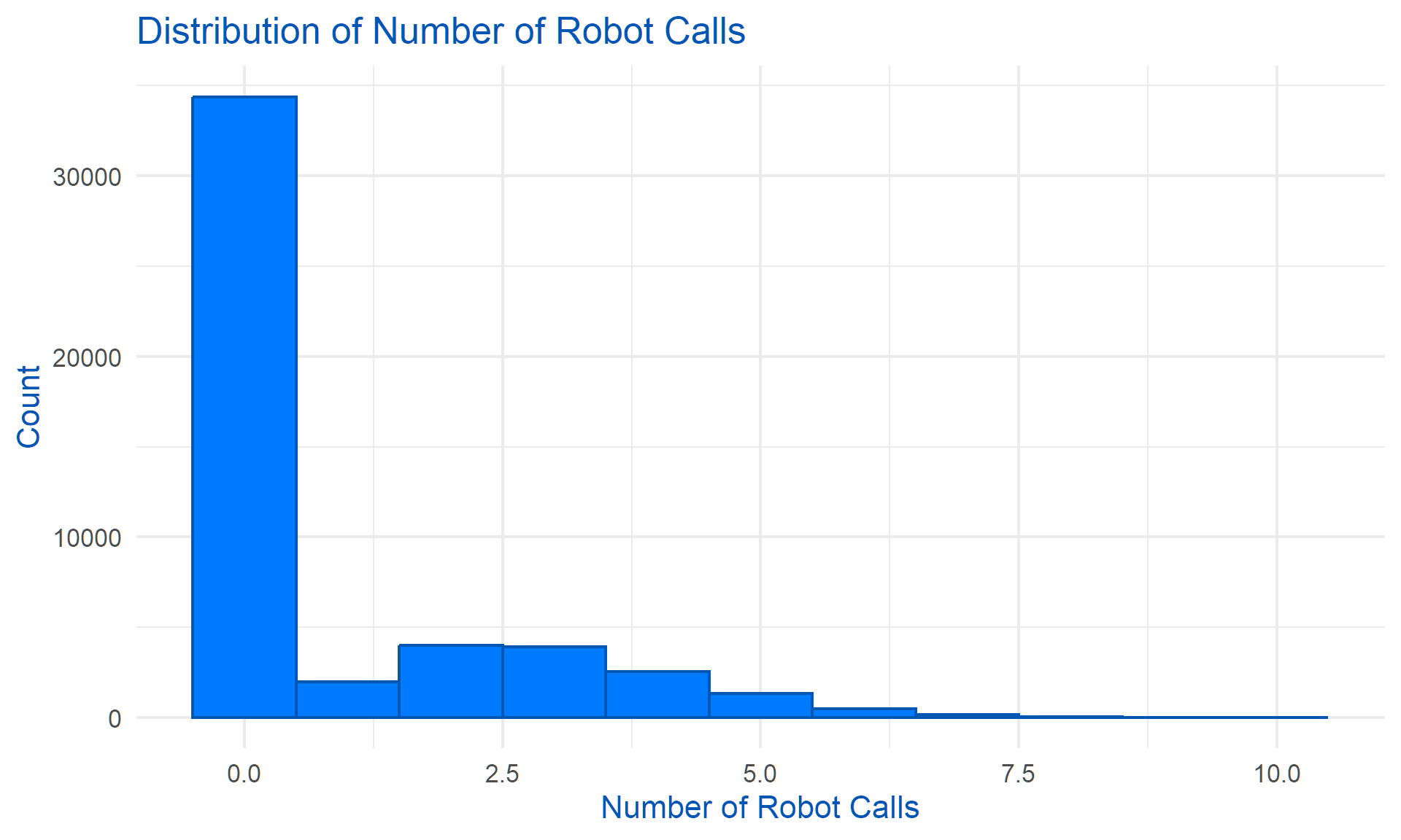
# 3. % Robot Calling by Purchase (enhanced legend)
df |>
  group_by(purchase) |>
  summarise(pct_robot_calling = mean(robot_calling, na.rm = TRUE)) |>
  ggplot(aes(x = factor(purchase, labels = c("No", "Yes")), y = pct_robot_calling)) +
  geom_bar(stat = "identity", fill = "#007bff") +
  theme_minimal(base_size = 16) +
  labs(title = "% Robot Calling by Purchase Outcome", x = "Purchase", y = "Proportion Robot Calls") +
  theme(text = element_text(color = "#0056b3"),
        legend.title = element_blank())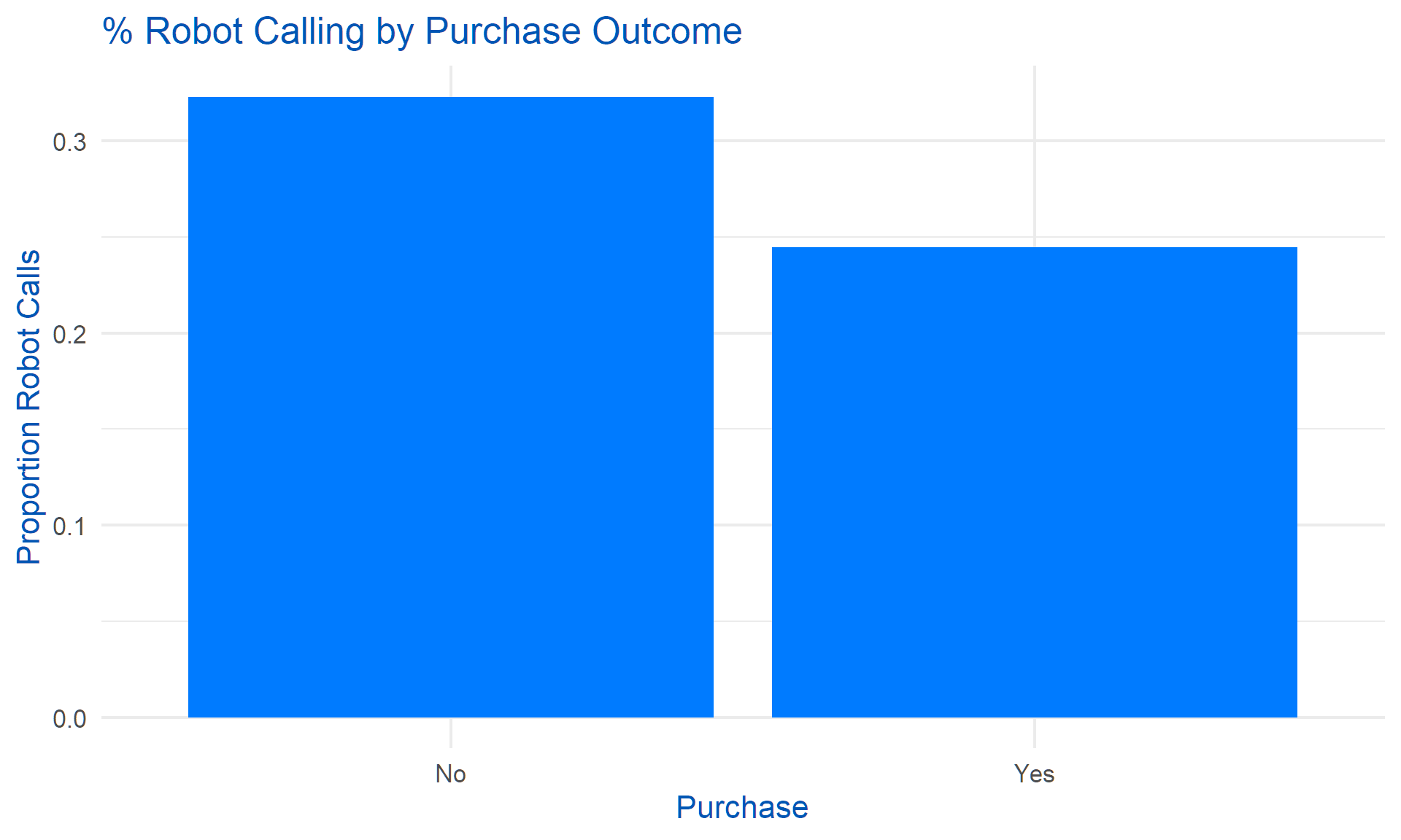
# 4. % Robot Calling by Marital Status (enhanced legend)
df |>
  group_by(marital_status) |>
  summarise(pct_robot_calling = mean(robot_calling, na.rm = TRUE)) |>
  ggplot(aes(x = marital_status, y = pct_robot_calling)) +
  geom_bar(stat = "identity", fill = "#007bff") +
  coord_flip() +
  theme_minimal(base_size = 16) +
  labs(title = "% Robot Calling by Marital Status", x = "Marital Status", y = "Proportion Robot Calls") +
  theme(text = element_text(color = "#0056b3"),
        legend.title = element_blank())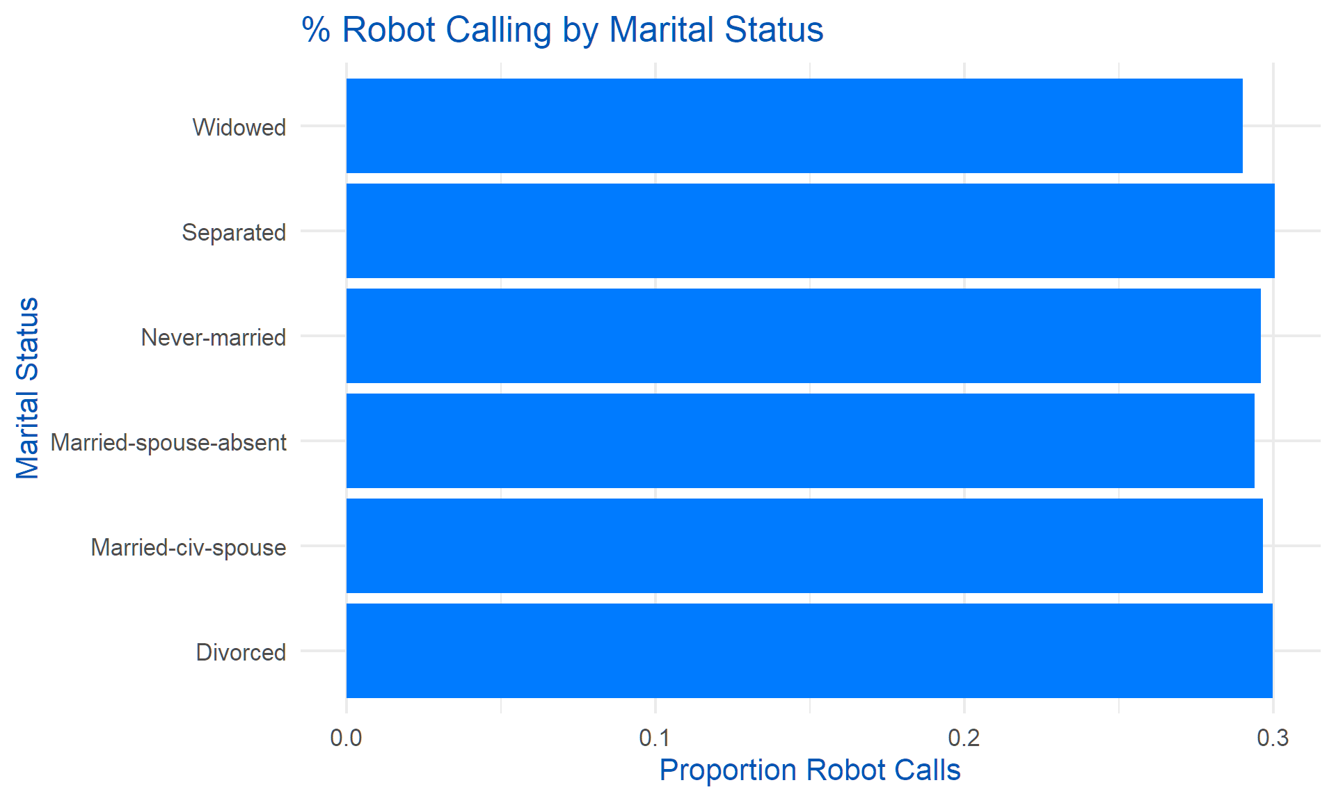
# 5. % Robot Calling by Occupation (enhanced legend)
df |>
  group_by(occupation) |>
  summarise(pct_robot_calling = mean(robot_calling, na.rm = TRUE)) |>
  ggplot(aes(x = occupation, y = pct_robot_calling)) +
  geom_bar(stat = "identity", fill = "#007bff") +
  coord_flip() +
  theme_minimal(base_size = 16) +
  labs(title = "% Robot Calling by Occupation Group", x = "Occupation", y = "Proportion Robot Calls") +
  theme(text = element_text(color = "#0056b3"),
        legend.title = element_blank())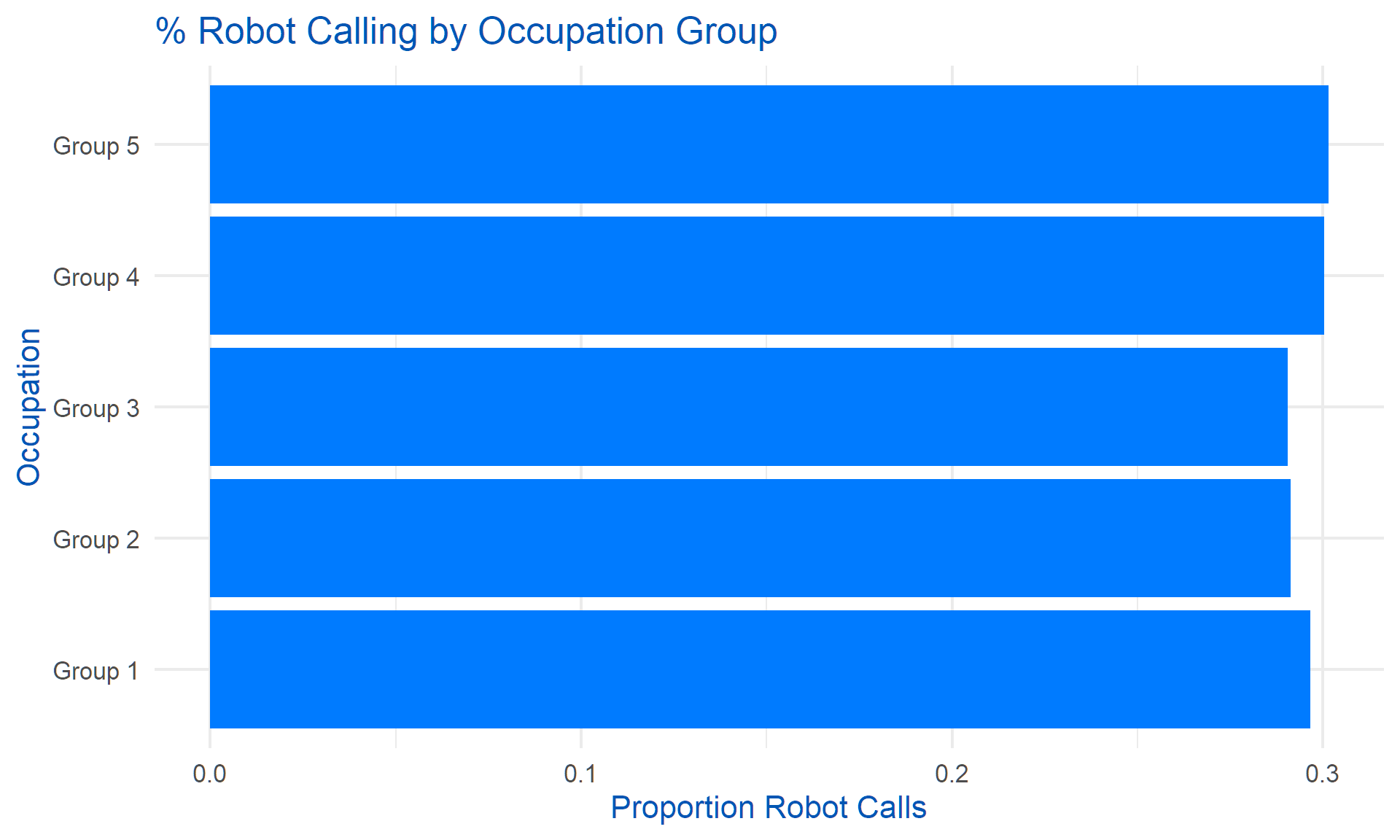
# 6. Boxplot of Robot Calls by Purchase (enhanced legend)
df |>
  ggplot(aes(x = factor(purchase, labels = c("No", "Yes")), y = number_of_robot_calls)) +
  geom_boxplot(fill = "#007bff") +
  theme_minimal(base_size = 16) +
  labs(title = "Number of Robot Calls by Purchase Outcome", x = "Purchase", y = "Number of Robot Calls") +
  theme(text = element_text(color = "#0056b3"),
        legend.title = element_blank())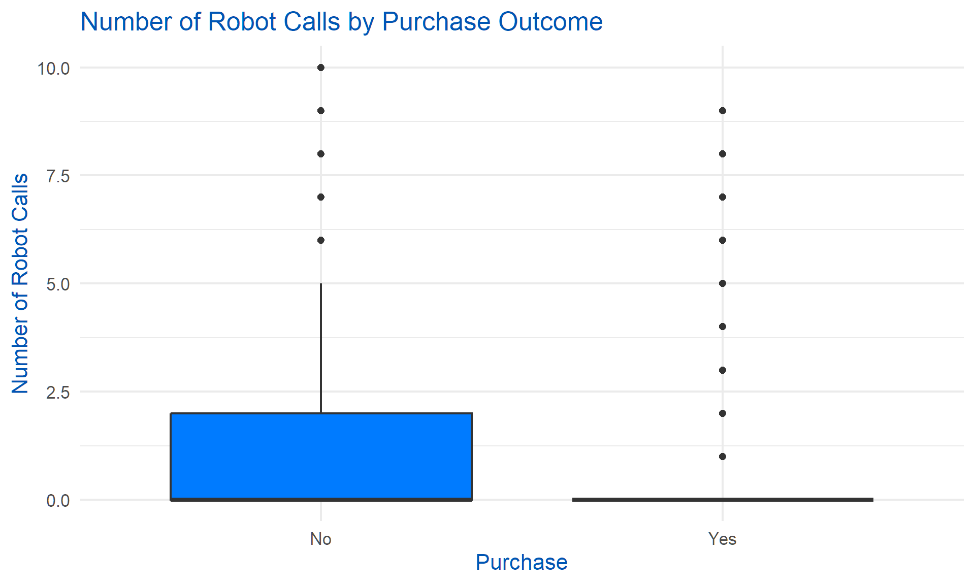
# 7. % Robot Calling by GDPR (enhanced legend)
df |>
  group_by(GDPR_applies) |>
  summarise(pct_robot_calling = mean(robot_calling, na.rm = TRUE)) |>
  ggplot(aes(x = factor(GDPR_applies, labels = c("No", "Yes")), y = pct_robot_calling)) +
  geom_bar(stat = "identity", fill = "#dc3545") +
  theme_minimal(base_size = 16) +
  labs(title = "% Robot Calling by GDPR Applicability", x = "GDPR Applies", y = "Proportion Robot Calls") +
  theme(text = element_text(color = "#0056b3"),
        legend.title = element_blank())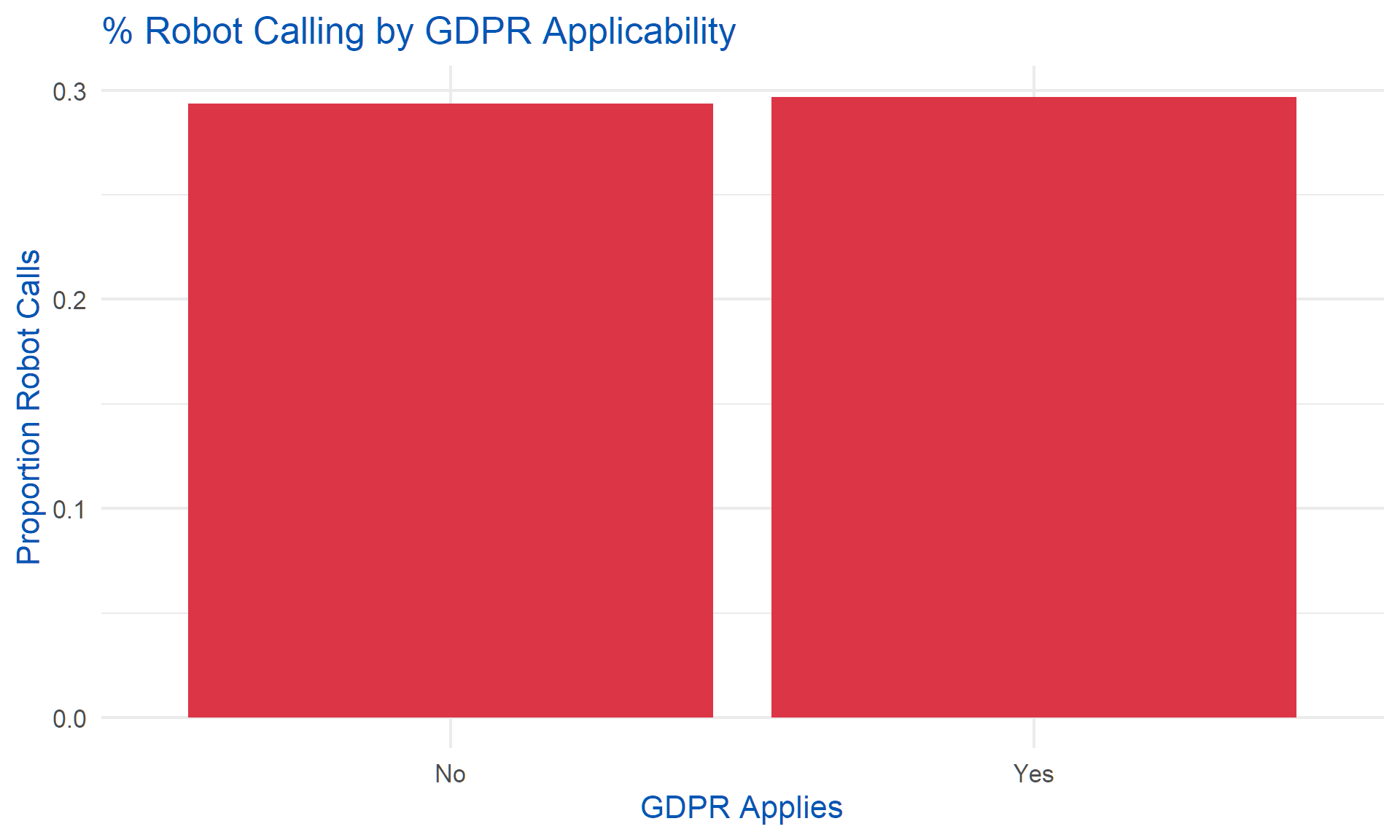
# 8. % Robot Calling by Age Group (enhanced legend)
df |>
  mutate(age_bin = cut(age, breaks = seq(15, 95, by = 10))) |>
  group_by(age_bin) |>
  summarise(pct_robot_calling = mean(robot_calling, na.rm = TRUE)) |>
  ggplot(aes(x = age_bin, y = pct_robot_calling)) +
  geom_bar(stat = "identity", fill = "#007bff") +
  theme_minimal(base_size = 16) +
  labs(title = "% Robot Calling by Age Group", x = "Age Group", y = "Proportion Robot Calls") +
  theme(axis.text.x = element_text(angle = 45, hjust = 1, color = "#0056b3"),
        legend.title = element_blank())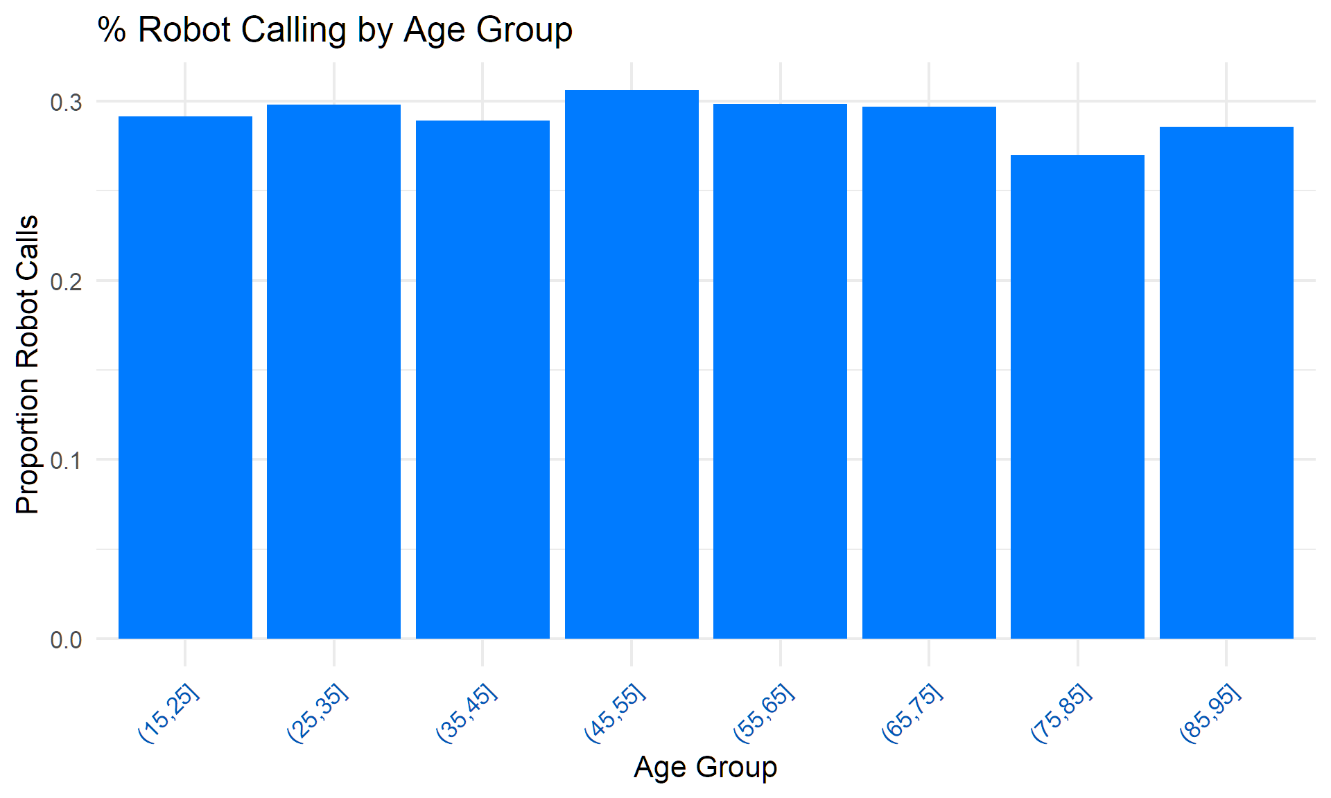
# New: % Robot Calling by Housing (added categorical)
df |>
  group_by(housing) |>
  summarise(pct_robot_calling = mean(robot_calling, na.rm = TRUE)) |>
  ggplot(aes(x = housing, y = pct_robot_calling)) +
  geom_bar(stat = "identity", fill = "#007bff") +
  coord_flip() +
  theme_minimal(base_size = 16) +
  labs(title = "% Robot Calling by Housing Loan", x = "Housing Loan", y = "Proportion Robot Calls") +
  theme(text = element_text(color = "#0056b3"),
        legend.title = element_blank())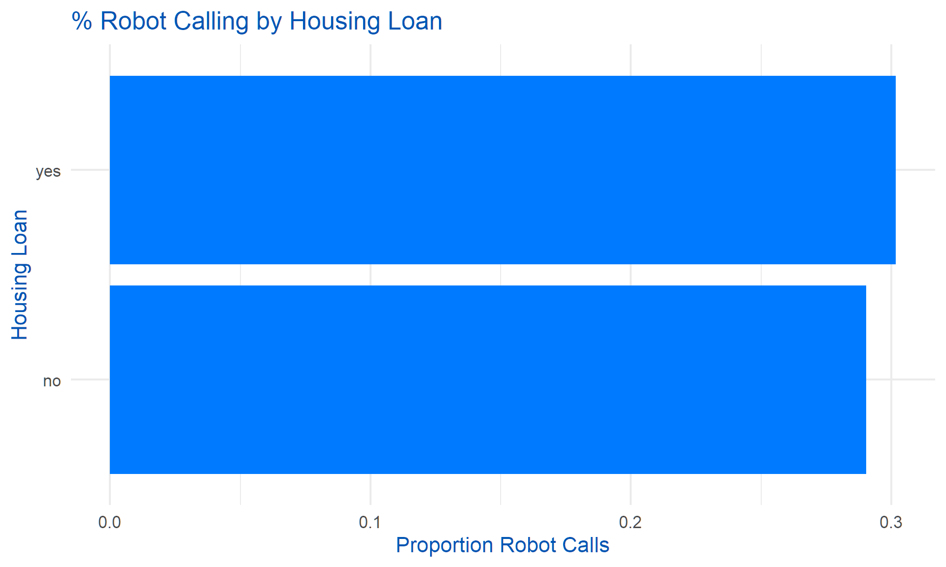
# New: % Robot Calling by Loan (added categorical)
df |>
  group_by(loan) |>
  summarise(pct_robot_calling = mean(robot_calling, na.rm = TRUE)) |>
  ggplot(aes(x = loan, y = pct_robot_calling)) +
  geom_bar(stat = "identity", fill = "#007bff") +
  coord_flip() +
  theme_minimal(base_size = 16) +
  labs(title = "% Robot Calling by Consumer Loan", x = "Consumer Loan", y = "Proportion Robot Calls") +
  theme(text = element_text(color = "#0056b3"),
        legend.title = element_blank())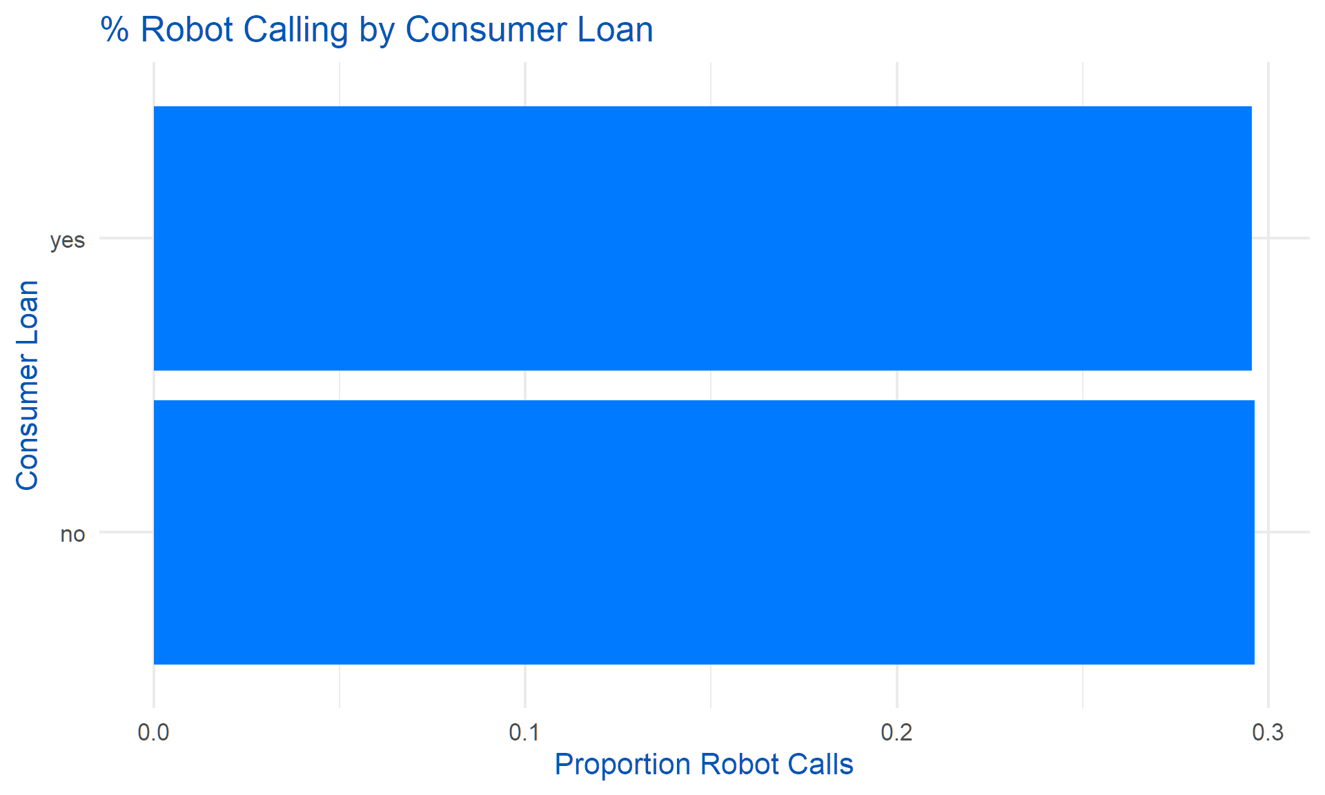
# New: % Robot Calling by Phone Type (added categorical)
df |>
  group_by(phone_type) |>
  summarise(pct_robot_calling = mean(robot_calling, na.rm = TRUE)) |>
  ggplot(aes(x = phone_type, y = pct_robot_calling)) +
  geom_bar(stat = "identity", fill = "#007bff") +
  coord_flip() +
  theme_minimal(base_size = 16) +
  labs(title = "% Robot Calling by Phone Type", x = "Phone Type", y = "Proportion Robot Calls") +
  theme(text = element_text(color = "#0056b3"),
        legend.title = element_blank())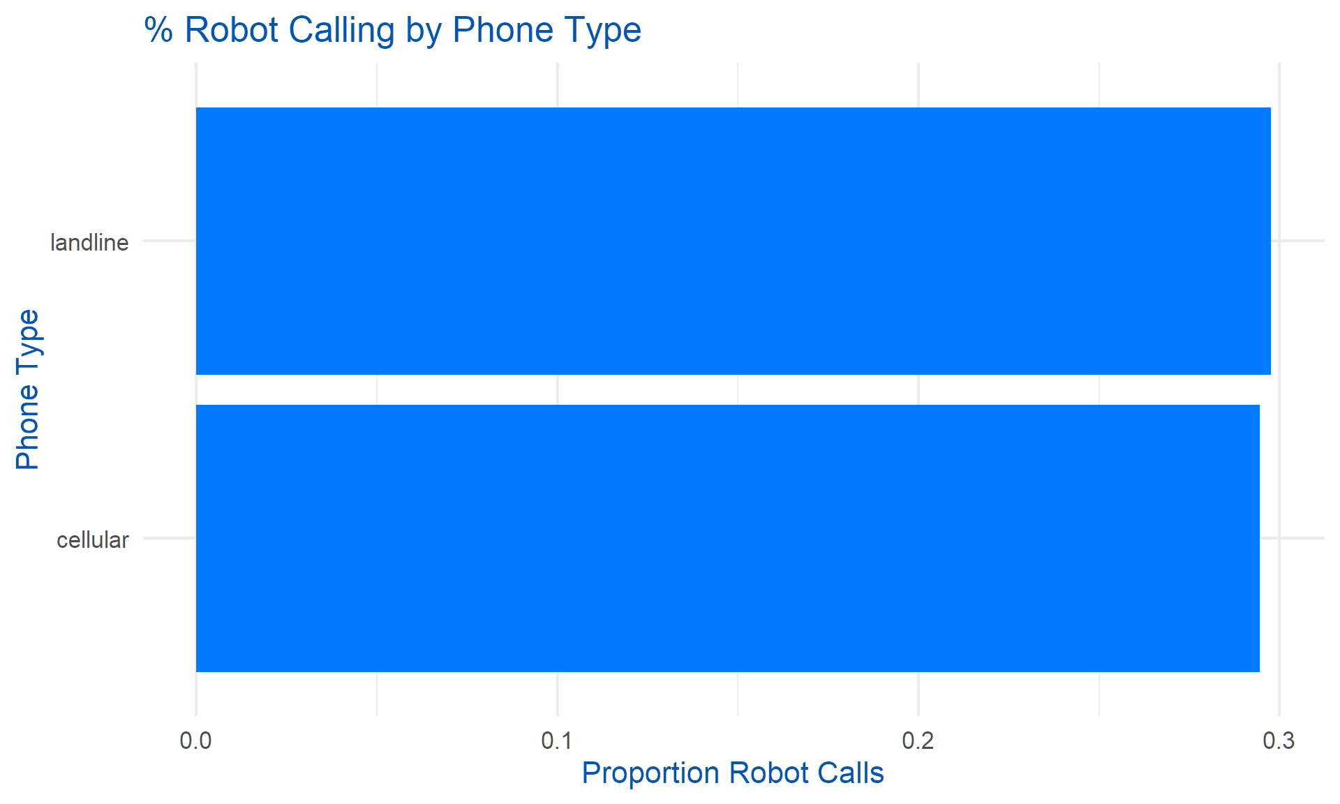
# New: % Robot Calling by Weekday (added categorical)
df |>
  group_by(weekday) |>
  summarise(pct_robot_calling = mean(robot_calling, na.rm = TRUE)) |>
  ggplot(aes(x = weekday, y = pct_robot_calling)) +
  geom_bar(stat = "identity", fill = "#007bff") +
  coord_flip() +
  theme_minimal(base_size = 16) +
  labs(title = "% Robot Calling by Weekday", x = "Weekday", y = "Proportion Robot Calls") +
  theme(text = element_text(color = "#0056b3"),
        legend.title = element_blank())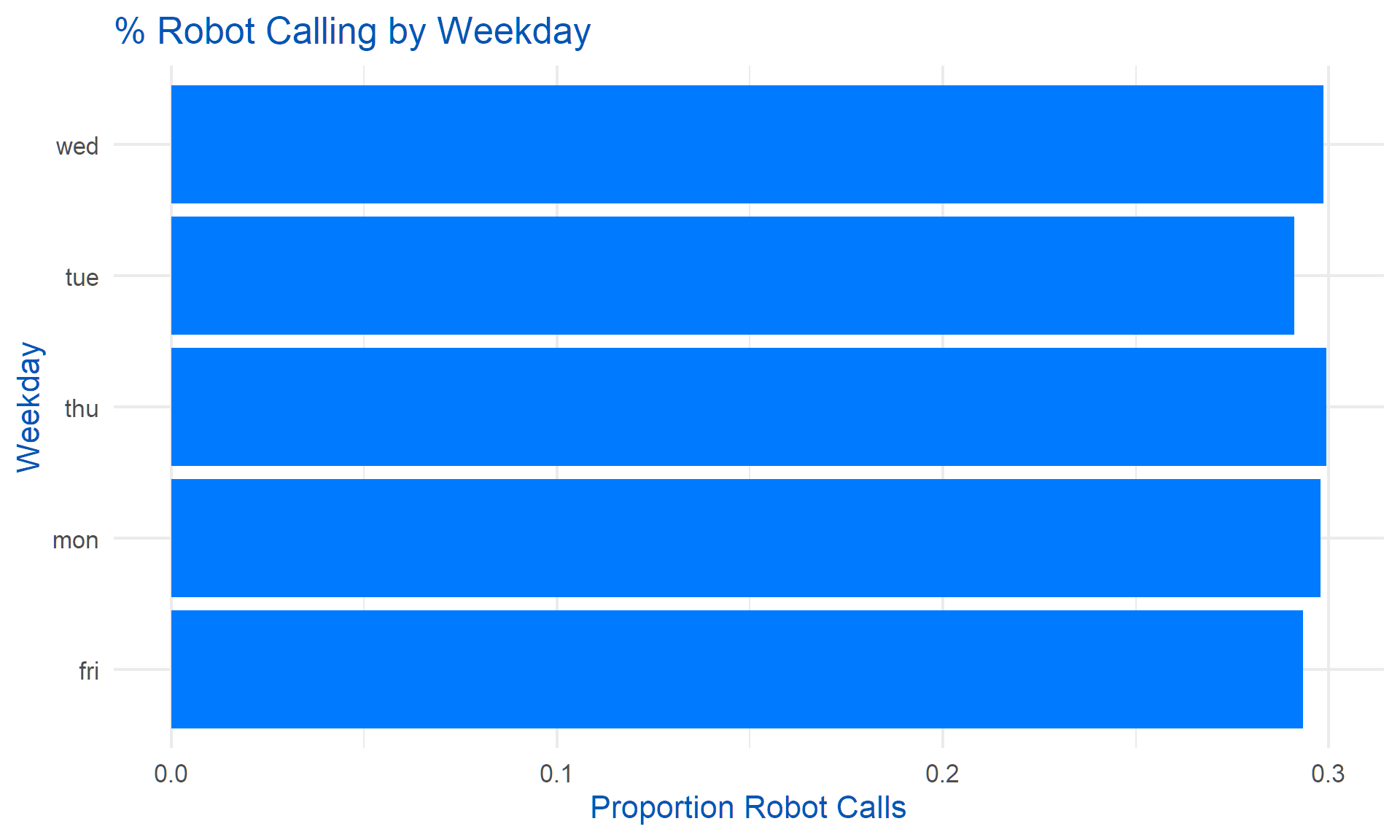
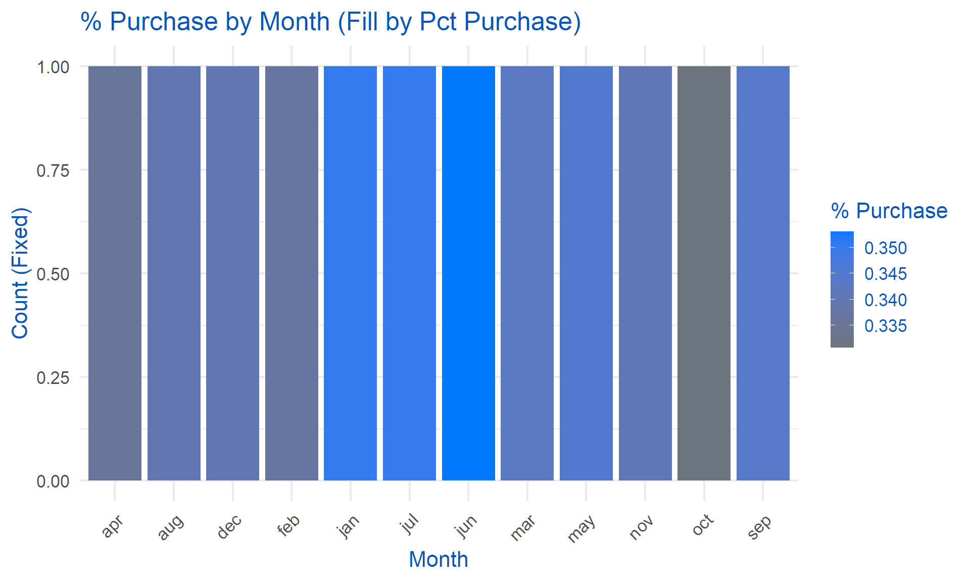
# For months: Pct purchase as fill/color
df |>
  group_by(month) |>
  summarise(pct_purchase = mean(purchase, na.rm = TRUE)) |>
  ggplot(aes(x = month, y = 1, fill = pct_purchase)) +
  geom_bar(stat = "identity") +
  scale_fill_gradient(low = "#6c757d", high = "#007bff") +  # Gray to blue
  theme_minimal(base_size = 16) +
  labs(title = "% Purchase by Month (Fill by Pct Purchase)", x = "Month", y = "Count (Fixed)", fill = "% Purchase") +
  theme(text = element_text(color = "#0056b3"),
        axis.text.x = element_text(angle = 45, hjust = 1))